1.REVIEW OF LINEAR EQUATIONS AND INEQUALITIES
1.1 Linear Equation in Two Variables
A linear equation in two variables x and y is of the form:
ax + by + c = 0
Where:
1.a, b, c → constants
2.x, y → variables
Represents a straight line in the plane.
1.2 Linear Inequality in Two Variables
A linear inequality in two variables can be of the form:
ax + by + c > 0
ax + by + c < 0
ax + by + c ≥ 0
ax + by + c ≤ 0
Example: x ≥ 3
1.Boundary line: x = 3
2.Region: all points to the right of the line
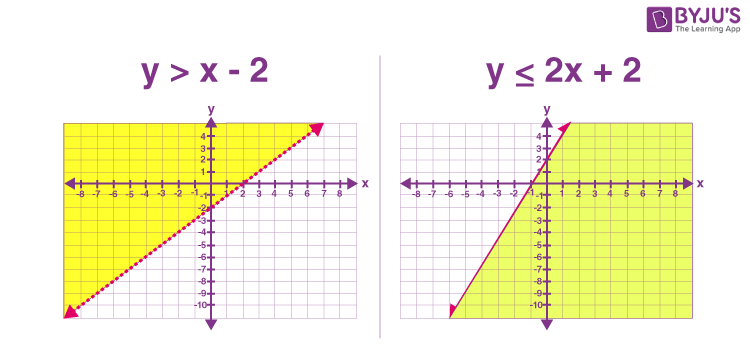
3.Solid line → ≥ or ≤
4.Dotted line → > or <
2.GRAPH OF LINEAR INEQUALITIES
Example 1: 2x + 3y ≥ 6
Boundary line: 2x + 3y = 6
| x | 0 | 3 | 6 |
|---|---|---|---|
| y | 2 | 0 | -2 |
1.Draw solid line
2.Test point (0,0): 2(0) + 3(0) ≥ 6 → 0 ≥ 6 → False
3.Shade opposite side of origin
Example 2: 2x − 3y < 6
Boundary line: 2x − 3y = 6
| x | 3 | 0 | -3 |
|---|---|---|---|
| y | 0 | -2 | -4 |
1.Draw dotted line
2.Test point (0,0): 0 − 0 < 6 → True
3.Shade region containing origin
Note: If the boundary passes through origin, test another point (1,0) or (0,1)
3.SYSTEM OF LINEAR INEQUALITIES
A system consists of two or more inequalities with a common solution region.
Example: x − 2y ≥ 4, 2x + y ≤ 8
Boundary Lines and Points:
| Line | x | y |
|---|---|---|
| x − 2y = 4 | 4 | 0 |
| 0 | -2 | |
| 2x + y = 8 | 0 | 8 |
| 4 | 0 |
Common shaded region = Feasible Region
4.LINEAR PROGRAMMING (L.P.)
Definition: A method to maximize or minimize a linear objective function under given constraints.
4.1 Basic Terms
1.Decision Variables → x, y
2.Objective Function → F = 4x − y
3.Constraints → e.g., 2x + 3y ≥ 6
4.Feasible Region → intersection of all constraints
5.Feasible Solution → any point in feasible region
6.Optimal Solution → occurs at vertices of feasible region
Important Rule: Maximum or minimum occurs at vertices only
5.STEPS TO SOLVE L.P. PROBLEMS
1.Identify decision variables and objective function
2.Convert constraints into equations (boundary lines)
3.Draw boundary lines on graph
4.Solid line if ≤ or ≥, Dotted line if < or >
5.Identify feasible region
6.Find vertices of feasible region
7.Evaluate objective function at each vertex
8.Select maximum and minimum value
6.EXAMPLE PROBLEMS
Example 1: Maximize F = 4x − y
Constraints: 2x + 3y ≥ 6, 2x − 3y ≤ 6, y ≤ 2
| Vertex | Coordinates | F = 4x − y |
|---|---|---|
| A | (3,0) | 12 |
| B | (6,2) | 22 (Max) |
| C | (0,2) | -2 (Min) |
Example 2: Max/Min Z = 2x + y
Constraints: x + y ≤ 6, x − y ≤ 4, x ≥ 0, y ≥ 0
| Vertex | Coordinates | Z = 2x + y |
|---|---|---|
| O | (0,0) | 0 (Min) |
| A | (4,0) | 8 |
| B | (5,1) | 11 (Max) |
| C | (0,6) | 6 |
Example 3: Minimize Z = 5x + 4y
Constraints: 2x + y ≥ 4, x + 2y ≥ 6, x ≥ 0, y ≥ 0
| Vertex | Coordinates | Z = 5x + 4y |
|---|---|---|
| A | (2,0) | 10 (Min) |
| B | (0,3) | 12 |
| C | (4/3,4/3) | 12 |
Example 4: Maximize P = 7x + 5y
Constraints: x + y ≤ 10, x ≤ 6, y ≤ 8, x ≥ 0, y ≥ 0
| Vertex | Coordinates | P = 7x + 5y |
|---|---|---|
| A | (0,0) | 0 |
| B | (6,0) | 42 |
| C | (6,4) | 62 (Max) |
| D | (2,8) | 54 |
7. Important Notes
1.Feasible region is always convex
2.Maximum/Minimum occurs only at vertices
3.Always test a point to decide shading
4.Solid line includes boundary, dotted line excludes boundary
5.Check non-negativity constraints (x ≥ 0, y ≥ 0)
Visit this link for further practice!!
https://besidedegree.com/exam/s/academic